Tauro

A cross-sectional statistical-arbitrage bot for crypto, built in early 2021 (and revisited in 2024) as my first machine learning project. The goal was to replicate a 2019 academic paper, then extend it with realistic execution costs. The extension failed. The way it failed turned out to be the most interesting part.

the paper

Fischer, Krauss & Deinert, Statistical Arbitrage in Cryptocurrency Markets. Journal of Risk and Financial Management, Feb 2019. Three researchers at Erlangen-Nürnberg ported a relative-value arbitrage technique that had previously been studied on US equities into the crypto markets.

The core idea is deceptively simple:

1. Every minute, take the top 40 coins by market cap.
2. For each coin, look at its returns over the past 1, 5, 10, 20… up to 1440 minutes (24 hours).
3. Train a random forest classifier to answer one question: will this coin’s return over the next 120 minutes be above or below the median of all 40 coins?
4. Long the three highest predicted probabilities, short the three lowest. Hold 120 minutes. Reverse.

The paper reports 7.1 bps per day, Sharpe 2.5, on an out-of-sample window from June–September 2018, after 15 bps per half-turn transaction costs. Importantly, this is market-neutral: profits come from one coin outperforming another, not from the market going up.

what I built

A research pipeline that downloads minute-bar price and volume data for the top 40 cryptocurrencies, computes features, trains the model, simulates trading over a held-out period, and reports performance. Everything below describes the backtest; the experiment never made it to live trading.

features

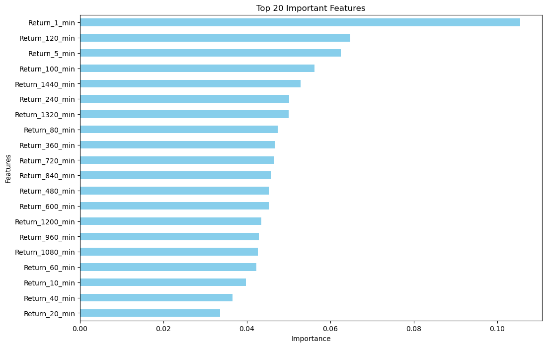
For each coin, at each minute, I compute log returns over twenty different lookbacks: 1, 5, 10, 20, 40, 60, 80, 100, 120 minutes, then every two hours out to 1440 minutes (24 hours). That’s the full feature vector: twenty numbers per coin per minute, no other engineered features, no order-book data, no sentiment.

target

A binary label: did this coin beat the cross-sectional median return over the next 122 minutes? The 122 instead of 120 is deliberate: there’s a one-minute gap between the signal time and the start of the return window, so the model can’t accidentally peek at information that wouldn’t be available at execution.

model

Random forest, 1,280 trees, max depth 15, with heavy regularization on the leaf size. That regularization was a deliberate departure from the paper, which used scikit-learn defaults. With roughly ten million training samples I was worried about trees overfitting onto noise, and the deeper splits weren’t contributing meaningfully to out-of-sample performance.

trading simulation

The simulator walks the out-of-sample period minute by minute, opens long positions on the three coins with the highest predicted probabilities and short positions on the three lowest, and closes them after 120 minutes, or earlier if a 28% adverse-move stop-loss triggers. (The stop was another deviation from the paper, which had no stops.) Signals are generated at the close of minute t and filled at the close of t+1 to avoid look-ahead bias, matching the paper’s execution gap. If a coin has no volume in the target minute, the trade is skipped.

performance analysis

A post-processing step applies fees (roughly 10 bps maker / 20 bps taker, matching what a retail account would have paid at the time), compounds capital across trades, and produces the cumulative-return and feature-importance plots that I’d then stare at trying to figure out why nothing worked.

what I changed from the paper

Component	Paper	My version
Data source	cryptocompare aggregate	direct from a major exchange
Return type	simple	log
Lookbacks	starts at 20 min	added 1, 5, 10 min
RF size	1,000 trees	1,280 trees
RF regularization	defaults	heavy (high min-split, high min-leaf)
Volatility stops	none	28% adverse-move stop
Baseline	logistic regression	dropped
Capital allocation	120 equal slots	compounding adjusted capital
Fees	15 bps half-turn	10/20 bps maker/taker
Test period	Jun–Sep 2018	early 2024

what happened

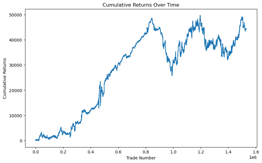
The paper’s strategy is a relative-value bet. In the paper’s 2018 window, the crypto market was in a sustained drawdown. The short leg of the portfolio (the flop-3 coins) carried the bulk of the alpha because most things were going down. The long leg was essentially flat.

In my 2024 backtest, the regime had completely flipped. Crypto was deep in a bull market. The longs were profitable, significantly so, but the shorts bled money continuously. The market-neutral premise broke: when the entire cross-section is drifting upward, “below-median” still means “going up, just less,” and you lose money shorting it.

Combine that with fees compounding on both legs of every round-trip trade, and the net was negative.

the deeper problem

Here’s the part that took me longer to see, and that I think is the real lesson.

The paper’s own Table 3 is a sensitivity analysis on execution timing. With no execution gap, the strategy makes 20.5 bps per round-trip. Delay execution by one minute (the paper’s published number): 3.8 bps. Two minutes: 2.4 bps. Three minutes: 1.6 bps. Four minutes: 0.9 bps, no longer statistically significant. Five minutes: zero.

The entire effect lives inside a three-minute window after signal generation. The paper authors flag this themselves: “fast execution after signal generation is paramount to the success of such a strategy.”

So the strategy isn’t really alpha in the sense of “we found a pattern the market hasn’t priced.” It’s a microstructural artifact: short-term mean reversion that the market does close, but takes a few minutes to do it. To capture it in production you’d need colocated execution, sub-100ms latency, and confidence that order management won’t introduce variable delay. None of which a hobbyist with a retail brokerage account was going to deliver, which is part of why the project never made it past backtesting.

The fees test wasn’t really a fees test. It was a stress test of how tight the strategy’s operational envelope had to be, and it failed at exactly the point where the academic version of “after costs” met the practitioner version of “after costs and slippage and execution variability.”

what I’d do differently

Looking at this two years later, a few things stand out:

• The compounding capital model makes the dollar P&L hard to interpret. Early trades are tiny, late trades are huge. I should have reported basis points per trade like the paper did, not raw dollars.
• No baseline. The paper compares the random forest to a logistic regression. Dropping the baseline made it impossible to tell whether the random forest was doing anything a linear model wouldn’t have done on its own.
• The 28% stop-loss is too wide to matter. A position needs a near-catastrophic move to hit it. Either it should have been tighter, something like 2× ATR, or removed entirely.
• No walk-forward validation. A two-thirds / one-third chronological split is fine for replicating the paper, but a real strategy needs rolling retraining to handle regime changes.

But mostly: I learned that “does it work after fees” is the only question that matters in algorithmic trading, and that academic backtests almost always describe a frictionless world that doesn’t survive contact with a real exchange.