Beating the Closing Line

For about a year I ran an NFL betting research project. This writeup covers the data and modeling half: a four-source pipeline that produces season-long parquet feature files, three custom team-quality metrics, and an XGBoost regressor that tries to predict the systematic error in the closing spread line. The companion agent that turned all of this into natural-language answers is covered separately: an NFL analyst agent.

The headline finding: 1,267 bets across the 2023, 2024, and 2025 seasons, 53.12% win rate, +19.6 units at standard -110 vig (1.41% ROI). Marginal positive expectation, edge concentrated entirely in underdogs. Honest version of “it works”: yes, but operationally too thin to scale, and how it works is more interesting than the headline number.

the pipeline

Four data sources, normalized into one SQLite database and then aggregated into a small set of master parquet files.

nflreadpy ───────►  raw play-by-play, player stats, team stats
                       │
Action Network ───►  consensus injury reports (scraped)
                       │
The Odds API ────►  live betting lines and prop markets
                       │
Google Sheets ───►  hand-graded weekly player grades
                       │
                       ▼
                 SQLite (nfl_data.db)
                       │
                       ▼
                 ETL + feature engineering
                       │
                       ▼
              processed/*.parquet
                       │
                       ▼
              Vercel Blob (hash-cached upload)

A note on nflreadpy: this whole project starts with a gift, and the gift has a backstory. The first version of the pipeline was a hand-rolled Yahoo Sports scraper that walked the weekly schedules and pulled box scores. Brittle, slow, but it worked. I shelved the project for a while, and when I fired it back up Yahoo had conveniently rolled out anti-scraping measures during the exact window I was offline. The harness no longer worked. The path forward was either an arms race with Yahoo’s bot detection or a complete rewrite, and that’s when I found nflreadpy.

nflreadpy is the Python port of nflreadr, both maintained as part of nflverse, a community-driven ecosystem of NFL data packages. It wraps the official NFL play-by-play feed, weekly rosters, schedules, weekly player stats, and Next Gen Stats (the ESPN tracking data that’s usually paywalled) into clean Polars dataframes that convert to pandas in one method call. Sensible caching, mid-game updates, excellent documentation, free and open source. The data-acquisition part of my pipeline became six function calls; the other 400+ lines of nflreadpy_update.py are downstream cleaning, joining, and SQLite insertion I wrote on top of what nflreadpy hands me, and they’re cleaner than the Yahoo scraper ever was because the upstream data is structured to begin with. Anything in this writeup that looks like it has good underlying data has good underlying data because of nflverse and the maintainers behind it. The Yahoo update almost certainly saved me from continuing with an inferior pipeline.

The hash-caching layer matters more than it looks. The pipeline runs on a cron, regenerates everything, computes an MD5 of each output file, compares against a .upload_cache.json keyed by blob path, and only uploads files whose hash has changed. The typical run touches maybe 5% of the files. The other 95% are immutable: a 2021 game’s box score doesn’t change after the game is final, and the prior season’s master parquet is fixed for the rest of recorded history. Vercel Blob charges per write, so caching brings the upload bill from “would notice on the credit card” to “rounding error.”

This wasn’t critical at hobbyist scale, but it’s the kind of optimization that decides whether a public product is viable. A live betting service would run this pipeline several times a day during the season (post-injury-report, post-game, pre-kickoff for line movement), every run regenerating the full dataset to be safe. Without hash-checking, every run re-uploads everything. With it, each run pushes roughly one-twentieth of that volume. Multiply by 17 weeks of football, several runs per day, and a real user base reading off the same blob store, and the difference between those two regimes is a meaningful line item on the monthly bill rather than a rounding error. The “static tail, moving head” pattern (historical record is immutable, only the active window updates) shows up in a lot of data pipelines; whenever it does, hash-before-write is one of the highest-leverage optimizations available.

Output is a small set of master parquets at game, team-game, team-season, player-game, and player-season grain, plus a context bundle (coaches, rosters, draft picks). The downstream model and the agent both load these directly from the blob URL at startup. Google Sheets is the one source that doesn’t fit the parquet-master pattern: it feeds the agent’s player-prop logic and is covered in the agent writeup.

three custom metrics

The model uses standard NFL features (EPA per play, yards per attempt, sack rates) plus three custom ones that I’d build into any future pipeline.

Team Edge Scoring

A composite power rating scaled 50-100, summarizing how good a team is at passing offense, rushing offense, pass defense, and rush defense, then rolled into total offense, total defense, and total team. Rollup weights are deliberate: passing is 60% of total offense, pass defense is 60% of total defense, and offense and defense are 50/50 in the team score.

The thing that makes it useful rather than just another rating: it’s calculated point-in-time. Week 5 ranks are computed only against the distribution of weeks 1 through 4 from that season. No future information leaks into the historical record. This was the trickiest part of the codebase to get right, and I rebuilt it twice after discovering subtle leakage that was inflating backtest results.

The inputs are 12 base metrics ranked into percentiles each week, then weighted into the composites:

• pass offense: passing EPA (50%), yards per pass (30%), sack rate (20%)
• rush offense: rushing EPA (60%), yards per rush (40%)
• pass defense: yards per pass attempt allowed (50%), sack rate (30%), takeaways (20%)
• rush defense: yards per rush allowed (60%), net rushing yards allowed (40%)

middle-eight net points

Net scoring in the last four minutes of the first half and first four minutes of the second half. A well-known concept in NFL handicapping circles. Teams that systematically dominate these windows tend to be better-coached than their season totals suggest, because both windows reward time management, in-game adjustments, and discipline. But I haven’t seen it published as a model feature anywhere.

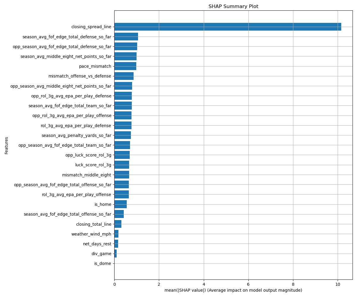
This ended up being one of the model’s higher-importance features, particularly in the mismatch_middle_eight interaction (your team’s middle-eight minus your opponent’s).

luck score

Actual wins minus Pythagorean expected wins. Standard idea borrowed from baseball sabermetrics: a team that wins more close games than their points-scored versus points-allowed ratio would predict is “lucky,” and luck regresses. A team carrying a few games of luck into a tough matchup is a signal to fade.

Computed at the season level, then converted to a rolling 3-game version for the model’s momentum features.

the model

XGBoost regression. Target is spread_error, the residual between actual game margin and the closing spread line.

Predicting the line’s bias rather than the game outcome directly is the only thing that can produce edge: the closing line already incorporates everything the betting market knows. Predicting the deviation from the line is predicting where the market is systematically wrong, not predicting football.

features

Bucket	What it captures	Examples
CONTROL	Market context + team fundamentals	closing spread/total, is_home, is_dome, wind, days rest, divisional game, Edge Scoring for both teams
MARKET_SENTIMENT	Sharp money indicators	money% minus bets% on spread, moneyline, total
MOMENTUM	Rolling 3-game form	rolling EPA per play offense/defense, rolling luck score, same for opponent
INTERACTION	Matchup mismatches	offense Edge Score minus opponent defense Edge Score, pace mismatch, middle-eight mismatch

The MARKET_SENTIMENT bucket sounds clever but turned out to be barely additive in feature importance, and I cut it from the final feature set. The signal it carries (sharp money moving lines) is already priced into the closing line by the time you observe it.

hyperparameters

• XGBRegressor, max_depth=4. Shallow trees on purpose: deeper trees memorize the small training set.
• n_estimators=2000 with early_stopping_rounds=50 on a 10% chronological validation slice
• learning_rate=0.05, subsample=0.8, colsample_bytree=0.8
• Final model trained on every available season; per-week predictions trained on everything chronologically before that week

validation

Multi-season walk-forward. The initial training window is 2021-2022 combined. Then for every week of 2023, 2024, and 2025, the model is retrained on the initial window plus every game chronologically prior to that week, and predictions are made on that week’s slate only. Computationally heavy (one retrain per week, 17 weeks per season, 3 seasons) but the only methodology that doesn’t leak future information into the past. For a time-series problem, it’s the only number I trust.

results

Across 2023-2025: 1,267 bets, 53.12% win rate, +19.6 units, 1.41% ROI. Breakeven at -110 vig is 52.38%, so this is real, but the interesting structure is in the confidence-tiered breakdown:

Predicted edge (points)	Tier	Bets	Win rate	ROI
under -14.0	Massive Strong Favorite	116	49.14%	-6.19%
-14.0 to -10.0	Super Strong Favorite	111	52.25%	-0.25%
-10.0 to -7.0	Very Strong Favorite	144	40.97%	-21.78%
-7.0 to -5.0	Strong Favorite	93	45.16%	-13.78%
-5.0 to -3.0	Medium Favorite	97	52.58%	+0.37%
-3.0 to -1.5	Weak Favorite	75	46.67%	-10.91%
1.5 to 3.0	Weak Underdog	74	58.11%	+10.93%
3.0 to 5.0	Medium Underdog	105	55.24%	+5.45%
5.0 to 7.0	Strong Underdog	84	51.19%	-2.27%
7.0 to 10.0	Very Strong Underdog	122	59.84%	+14.23%
10.0 to 14.0	Super Strong Underdog	111	52.25%	-0.25%
over 14.0	Massive Strong Underdog	135	47.41%	-9.49%

The model is essentially an underdog-spotter. Favorite-side bets, where the model agreed with the market that team X should win by 7+ points, mostly bled money. Underdog-side bets, especially the 7-10 point range, are where almost all of the realized edge lives.

a note on efficiency

NFL closing lines are widely considered the most efficient market in US sports. Sportsbooks like Pinnacle and Circa accept the largest bets from professional bettors, then adjust their lines toward where that money flows; by kickoff, the published line reflects the consensus of the most informed money in the market. Industry research treats beating the closing line over a large sample as the gold-standard test of skill in sports betting, and the consensus is that even sharp professionals rarely clear the closing line by more than 1 to 3% long-term.

This experiment cleared it by 1.41% over 1,267 bets. Directionally that’s in the right neighborhood, but it’s also barely outside the noise envelope. At a breakeven win rate of 52.38% the standard deviation of 1,267 binomial trials is roughly 9 wins, and the model produced about 9 or 10 wins above breakeven. z ≈ 0.5, one-tailed p ≈ 0.30. By any conventional significance test, you cannot reject the null hypothesis that the headline number is pure variance around a breakeven baseline.

The fair reading is that the aggregate result is statistically indistinguishable from noise. The tier breakdown is suggestive, especially the very-strong-favorite bucket where the model loses badly enough (z ≈ -2.7) to be hard to explain by chance even after correcting for testing across 12 tiers, but with that many tiers you’d expect at least one to look extreme. What’s actually defensible from this project isn’t “I beat the market.” It’s “I built a rigorous walk-forward pipeline that landed in the range where small real edges live, on a market famously hard to beat.” The engineering is the artifact; the ROI is the test, and the test came back inconclusive.

the open puzzle

Why does the model lose on favorites and win on underdogs?

Two non-exclusive hypotheses, neither of which I’ve fully nailed down:

1. The market systematically overprices public favorites. Casual money flows toward big-name teams, oddsmakers shade the line a half-point toward the public to balance their book, and the closing line is biased against the favorite. The model picks up on the bias and bets the underdog, profitably. Favorite-side picks, where the model agrees with the public, are by construction less informed.

2. The model is missing a feature that would help on favorite-side games. Possibly something about how favorites behave when leading (clock management, garbage-time stats inflating the rolling averages). Possibly something about coaching decisions in high-leverage situations. I tried adding pass_rate_leading and a handful of others; none moved the needle materially.

There’s a third possibility that I think is real but harder to test: 1,267 bets sounds like a lot, but for a single-regime sample it’s still close enough to noise that the favorite/underdog asymmetry could be a 2023-2025 artifact (the league has been unusually high-scoring and underdog-friendly in that window), and a future regime could reverse it. Walk-forward validation guards against lookahead but not against regime shift.

what I’d do differently

• Continuous injury severity. The current pipeline treats injuries as a categorical (out / questionable / probable). A regression of historical injury-status against actual snap counts would produce a continuous “expected snap share” feature that’s much richer.
• Separate model for high-line-movement games. Sharps tend to act early, line movement of 1.5+ points before kickoff is informative, and the model currently treats it as just another feature. A submodel trained only on heavy-movement games is worth a real test.
• Switch the target. Predicting spread_error is a regression on margin, but the actual decision is binary (bet or don’t, which side). A classifier on “is there a +EV bet here” using the same features might be more robust because the objective lines up exactly with the betting decision instead of being a proxy.

The 1.41% ROI is real, walk-forward, and reproducible. It’s also too thin to ever cover the operational overhead of a live betting product: the vig on a -110 bet is roughly 4.55% of the staked amount, and the model captures less than a third of that as edge. That’s the part the headline number doesn’t quite show, and it’s part of why I shut the project down.